Ehrenfest theorem

Quantum mechanics
$\Delta x\, \Delta p \ge \frac{\hbar}{2}$ Uncertainty principle
Introduction Glossary · History
Background Bra-ket notation · Classical mechanics Hamiltonian · Interference Old quantum theory
Fundamental concepts Complementarity · Decoherence Duality · Ehrenfest theorem Entanglement · Exclusion Measurement · Probability amplitude Nonlocality · Quantum state Superposition · Tunnelling Uncertainty · Wave function
Experiments Bell's inequality · Davisson–Germer Delayed choice quantum eraser Double-slit · Elitzur–Vaidman Popper · Quantum eraser Schrödinger's cat · Stern–Gerlach Wheeler's delayed choice
Formulations Formulations Heisenberg · Interaction Matrix mechanics · Schrödinger Sum over histories
Equations Dirac · Klein–Gordon Pauli · Rydberg Schrödinger
Interpretations Consciousness-caused Consistent histories Copenhagen · de Broglie–Bohm Ensemble · Hidden variables Many-worlds · Objective collapse Pondicherry · Quantum logic Relational · Stochastic Transactional
Advanced topics Quantum chaos · Quantum field theory Quantum information science Scattering theory
Scientists Bell · Bohm · Bohr · Born · Bose de Broglie · Dirac · Ehrenfest Everett · Feynman · Heisenberg Jordan · Kramers · von Neumann Pauli · Planck · Schrödinger Sommerfeld · Wien · Wigner

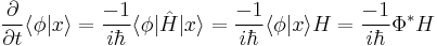
The Ehrenfest theorem, named after Paul Ehrenfest, the Austrian physicist and mathematician, relates the time derivative of the expectation value for a quantum mechanical operator to the commutator of that operator with the Hamiltonian of the system. It is

$\frac{d}{dt}\langle A\rangle = \frac{1}{i\hbar}\langle [A,H] \rangle%2B \left\langle \frac{\partial A}{\partial t}\right\rangle$

where A is some QM operator and $\langle A\rangle$ is its expectation value. Ehrenfest's theorem is obvious in the Heisenberg picture of quantum mechanics, where it is just the expectation value of the Heisenberg equation of motion.

Ehrenfest's theorem is closely related to Liouville's theorem from Hamiltonian mechanics, which involves the Poisson bracket instead of a commutator. In fact, it is a rule of thumb that a theorem in quantum mechanics which contains a commutator can be turned into a theorem in classical mechanics by changing the commutator into a Poisson bracket and multiplying by $i\hbar$ . This causes the operator expectation values to obey their corresponding classical equations of motion provided the Hamiltonian is at most quadratic in the coordinates and momenta. Otherwise, the equations still may hold approximately, provided fluctuations are small.

Derivation

Suppose some system is presently in a quantum state $\Phi$ . If we want to know the instantaneous time derivative of the expectation value of A, that is, by definition

$\frac{d}{dt}\langle A\rangle = \frac{d}{dt}\int \Phi^* A \Phi~dx^3 = \int \left( \frac{\partial \Phi^*}{\partial t} \right) A\Phi~dx^3 %2B \int \Phi^* \left( \frac{\partial A}{\partial t}\right) \Phi~dx^3 %2B\int \Phi^* A \left( \frac{\partial \Phi}{\partial t} \right) ~dx^3$

$= \int \left( \frac{\partial \Phi^*}{\partial t} \right) A\Phi~dx^3 %2B \left\langle \frac{\partial A}{\partial t}\right\rangle %2B \int \Phi^* A \left( \frac{\partial \Phi}{\partial t} \right) ~dx^3,$

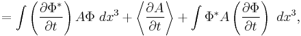
where we are integrating over all space. If we apply the Schrödinger equation, we find that

$\frac{\partial \Phi}{\partial t} = \frac{1}{i\hbar}H\Phi$

and

$\frac{\partial \Phi^*}{\partial t} = \frac{-1}{i\hbar}\Phi^*H^* = \frac{-1}{i\hbar}\Phi^*H.$ ^[1]

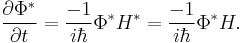
Notice $H=H^*$ because the Hamiltonian is hermitian. Placing this into the above equation we have

$\frac{d}{dt}\langle A\rangle = \frac{1}{i\hbar}\int \Phi^* (AH-HA) \Phi~dx^3 %2B \left\langle \frac{\partial A}{\partial t}\right\rangle = \frac{1}{i\hbar}\langle [A,H]\rangle %2B \left\langle \frac{\partial A}{\partial t}\right\rangle.$

Often (but not always) the operator A is time independent, so that its derivative is zero and we can ignore the last term.

General example

For the very general example of a massive particle moving in a potential, the Hamiltonian is simply

$H(x,p,t) = \frac{p^2}{2m} %2B V(x,t)$

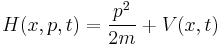
where $x$ is just the location of the particle. Suppose we wanted to know the instantaneous change in momentum $p$ . Using Ehrenfest's theorem, we have

$\frac{d}{dt}\langle p\rangle = \frac{1}{i\hbar}\langle [p,H]\rangle %2B \left\langle \frac{\partial p}{\partial t}\right\rangle = \frac{1}{i\hbar}\langle [p,V(x,t)]\rangle$

since the operator $p$ commutes with itself and has no time dependence.^[2] By expanding the right-hand-side, replacing p by $-i\hbar \nabla$ , we get

$\frac{d}{dt}\langle p\rangle = \int \Phi^* V(x,t)\nabla\Phi~dx^3 - \int \Phi^* \nabla (V(x,t)\Phi)~dx^3.$

After applying the product rule on the second term, we have

$\frac{d}{dt}\langle p\rangle = \int \Phi^* V(x,t)\nabla\Phi~dx^3 - \int \Phi^* (\nabla V(x,t))\Phi ~dx^3 - \int \Phi^* V(x,t)\nabla\Phi~dx^3$

$= - \int \Phi^* (\nabla V(x,t))\Phi ~dx^3$

$= \langle -\nabla V(x,t)\rangle = \langle F \rangle,$

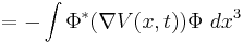
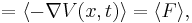
but we recognize this as Newton's second law. This is an example of the correspondence principle, the result manifests as Newton's second law in the case of having so many particles that the net motion is given exactly by the expectation value of a single particle.

Similarly we can obtain the instantaneous change in the position expectation value.

$\frac{d}{dt}\langle x\rangle = \frac{1}{i\hbar}\langle [x,H]\rangle %2B \left\langle \frac{\partial x}{\partial t}\right\rangle =$

$= \frac{1}{i\hbar}\langle [x,\frac{p^2}{2m} %2B V(x,t)]\rangle %2B 0 = \frac{1}{i\hbar}\langle [x,\frac{p^2}{2m}]\rangle =$

$= \frac{1}{i\hbar}\langle [x,\frac{p^2}{2m} %2B V(x,t)]\rangle = \frac{1}{i\hbar 2 m}\langle [x,p] \frac{d}{dp} p^2\rangle =$

$= \frac{1}{i\hbar 2 m}\langle i \hbar 2 p\rangle = \frac{1}{m}\langle p\rangle$

This result is again in accord with the classical equation.

Notes

^ In bra-ket notation

$\frac{\partial}{\partial t}\langle \phi |x\rangle =\frac{-1}{i\hbar}\langle \phi |\hat{H}|x\rangle =\frac{-1}{i\hbar}\langle \phi |x \rangle H=\frac{-1}{i\hbar}\Phi^*H$

where $\hat{H}$ is the Hamiltonian operator, and H is the Hamiltonian represented in coordinate space (as is the case in the derivation above). In other words, we applied the adjoint operation to the entire Schrödinger equation, which flipped the order of operations for H and $\Phi$ .
^ Although the expectation value of the momentum $\scriptstyle \langle p \rangle$ , which is a real-number-valued function of time, will have time dependence, the momentum operator $\scriptstyle p$ does not. Rather, the momentum operator is a constant linear operator on the Hilbert space of the system. The time dependence of the expectation value is due to the time evolution of the wavefunction for which the expectation value is calculated. An Ad hoc example of an operator which does have time dependence is $\scriptstyle x t^2$ , where $\scriptstyle x$ is the ordinary position operator and $\scriptstyle t$ is just the (non-operator) time.